As
shown in the Excel file, Howell
13-2, the
ANOVA analysis (in the ToolPac) yielded the following table:
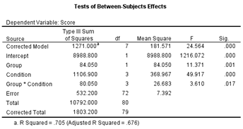
All
effects—Sample (Group), Columns (Condition), and the Group x Condition
interaction—were statistically significant at p < .05. (I provide a sample write-up later.)
For
the next analysis I used VassarStats
>
Two-Way Factorial ANOVA for Independent Samples.
Following the directions given there, I obtained the following. (Note that the
ANOVA summary table is the same as that for the Excel example.)
![]()
|
Data Entered |
||||
|
|
Col
1 |
Col
2 |
Col
3 |
Col
4 |
|
Row 1 |
9 |
7 |
11 |
12 |
|
Row 2 |
8 |
10 |
14 |
20 |
|
Row 3 |
--- |
--- |
--- |
--- |
|
Row 4 |
--- |
--- |
--- |
--- |
![]()
|
Summary Data |
Within each box: |
||||
|
|
C1 |
C2 |
C3 |
C4 |
Tot. |
|
R1 |
10 |
10 |
10 |
10 |
40 |
|
R2 |
10 |
10 |
10 |
10 |
40 |
|
R3 |
--- |
--- |
--- |
--- |
--- |
|
R4 |
--- |
--- |
--- |
--- |
--- |
|
Tot. |
20 |
20 |
20 |
20 |
80 |
![]()
|
ANOVA Summary |
|||||
|
Source |
SS |
df |
MS |
F |
P |
|
Rows |
84.05 |
1 |
84.05 |
11.37 |
0.0012 |
|
Columns |
1106.9 |
3 |
368.97 |
49.92 |
<.0001 |
|
r x c |
80.05 |
3 |
26.68 |
3.61 |
0.0173 |
|
Error |
532.2 |
72 |
7.39 |
||
|
Total |
1803.2 |
79 |
|||
![]()
|
Critical Values for the
Tukey HSD Test |
|||
|
HSD[.05] |
HSD[.01] |
HSD=the absolute [unsigned]
difference between any two means (row means, column means, or cell means)
required for significance at the designated level: HSD[.05] for the .05 level;
HSD[.01] for the .01 level. The HSD test between row means can be
meaningfully performed only if the row effect is significant; between
column means, only if the column effect is significant; and between cell
means, only if the interaction effect is significant. |
|
|
Rows [2] |
1.21 |
1.61 |
|
|
Columns [4] |
2.26 |
2.78 |
|
|
Cells [8] |
3.8 |
4.48 |
|
From
the third row of the Tot subsection of the Summary
Data table, the means of the four conditions are 6.75, 7.25, 12.9, and
15.5. From the Tukey HSD table we see that to
be statistically significant at p <.05
we need a difference between any two means to be at least 2.26 units. The
difference between means for Condition 1 and Condition 2 does not satisfy this
criterion. Hence we find no evidence that rhyming was any more effective than
counting. On the other hand the differences between Condition 3 and Condition 2
(an, of course, Condition 1) was statistically significant. The same can be said
about Condition 4 (vs Conditions 1 & 2). Also, the difference between
Condition 4 and Condition 3 is statistically significant.
There
is still a problem that needs to be addressed, however. The presences of a
significant interaction tells us that there is a differential effect of
Conditions depending upon which group, young or old, is examined. I will treat
this in the next analysis.
|
SPSS
Syntax for Analyzing Howell’s Table 13-2 *The commands for this first
analysis specify an overall 2x3 ANOVA. DATASET
ACTIVATE DataSet1. *Since the first analysis
yielded a significant Group (or Age) by Condition Interaction, we should
perform simple effects analyses within groups. This command splits the
data file by Group. SPLIT
FILE LAYERED BY Group. *The next set of commands
re-run the earlier analysis, only this time the analysis is computed once
for each group. Additionally, for each analysis, SPSS is instructed to
generate plots of means. UNIANOVA
Score BY Group Condition |
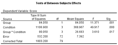
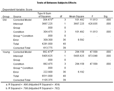
Again,
there is more information given in the table than we need. In addition to the Corrected
Model, Intercept, and Total
sources of variance, we do not need the Group and
Group * Condition source of variance since,
in simple effects, these are not factors. By double clicking on this table in
SPSS, the table can be edited to look like the following.
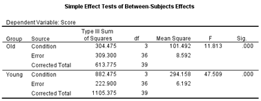
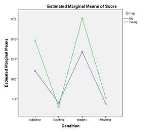
The
Condition effect is significant within both groups.
The
syntax also instructed SPSS to compute post hoc comparisons, using Tukey’s HSD
test. Since the data file was split on Group, these comparisons are performed
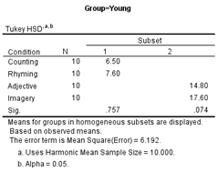
separately for each group. The post hoc analyses are summarized in a homogeneous
subsets table:
|
|
|